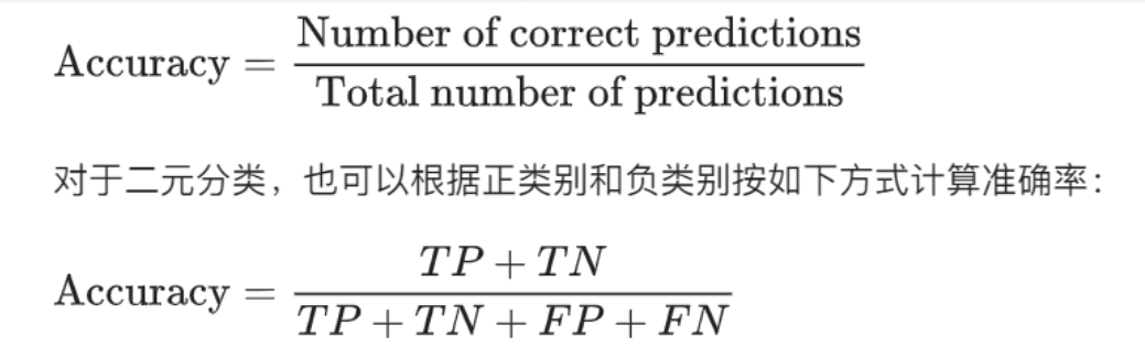
准确率 accuracy
当您使用分类不平衡的数据集(比如正类别标签和负类别标签的数量之间存在明显差异)时,单单准确率一项并不能反映全面情况 所以需要精确率和召回率
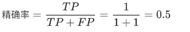
precision and recall
Precision:在被识别为正类别的样本中,确实为正类别的比例是多少?
ROC AUC
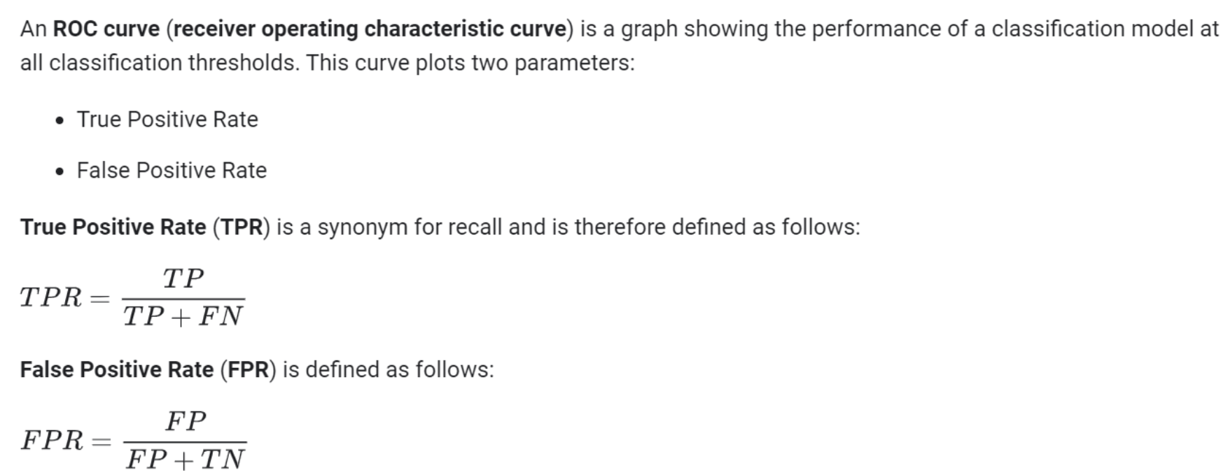
曲线下面积表示随机正类别(绿色)样本位于随机负类别(红色)样本右侧的概率。
曲线下面积因以下两个原因而比较实用:
- 曲线下面积的尺度不变。它测量预测的排名情况,而不是测量其绝对值。
- 曲线下面积的分类阈值不变。它测量模型预测的质量,而不考虑所选的分类阈值
L1, L2 正则化
L1 正则化可以让一些不必要的权重变为0,减少RAM消耗,和计算量,如果用L2话不能使得权重变为0,那么计算量依然是很大的。
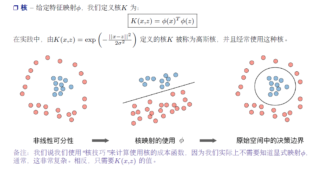
“非线性”意味着您无法使用形式为 b+w1x1+w2x2 的模型准确预测标签。也就是说,“决策面”不是直线。之前,我们了解了对非线性问题进行建模的一种可行方法
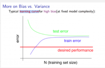
Learning Curves
Training an algorithm on a very few number of data points (such as 1, 2 or 3) will easily have 0 errors because we can always find a quadratic curve that touches exactly those number of points. Hence:
- As the training set gets larger, the error for a quadratic function increases.
- The error value will plateau out after a certain m, or training set size.
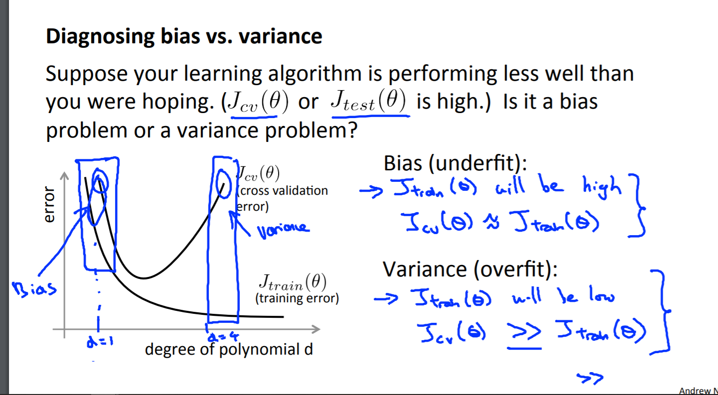
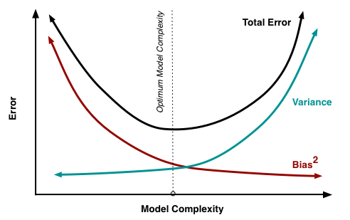
Experiencing high bias:
If a learning algorithm is suffering from high bias, getting more training data will not (by itself) help much.
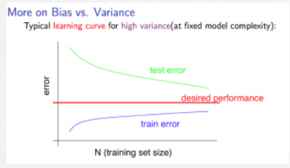
Experiencing high variance:
If a learning algorithm is suffering from high variance, getting more training data is likely to help.
Deal with High bias or high variance
- Getting more training examples: Fixes high variance
- Trying smaller sets of features: Fixes high variance
- Adding features: Fixes high bias
- Adding polynomial features: Fixes high bias
- Decreasing λ: Fixes high bias
- Increasing λ: Fixes high variance.
ML-Clustering-Unsupervised Learning: Introduction
Using these variables we can define our cost function:
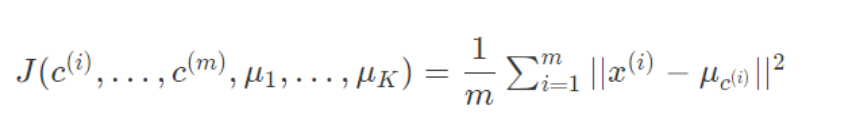
With k-means, it is not possible for the cost function to sometimes increase. It should always descend. K-means can get stuck in local optima. To decrease the chance of this happening,** you can run the algorithm on many different random initializations**. In cases where K<10 it is strongly recommended to run a loop of random initializations.
Choosing the Number of Clusters:
The elbow method: plot the cost J and the number of clusters K. The cost function should reduce as we increase the number of clusters, and then flatten out. Choose K at the point where the cost function starts to flatten out.
Note: J will always decrease as K is increased. The one exception is if k-means gets stuck at a bad local optimum.
Learning with Large Datasets
Stochastic Gradient Descent
This algorithm will only try to fit one training example at a time.
Mini-Batch Gradient Descent
Instead of using all m examples as in batch gradient descent, and instead of using only 1 example as in stochastic gradient descent, we will use some in-between number of examples b.
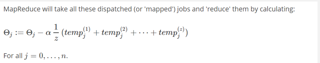
Map Reduce and Data Parallelism
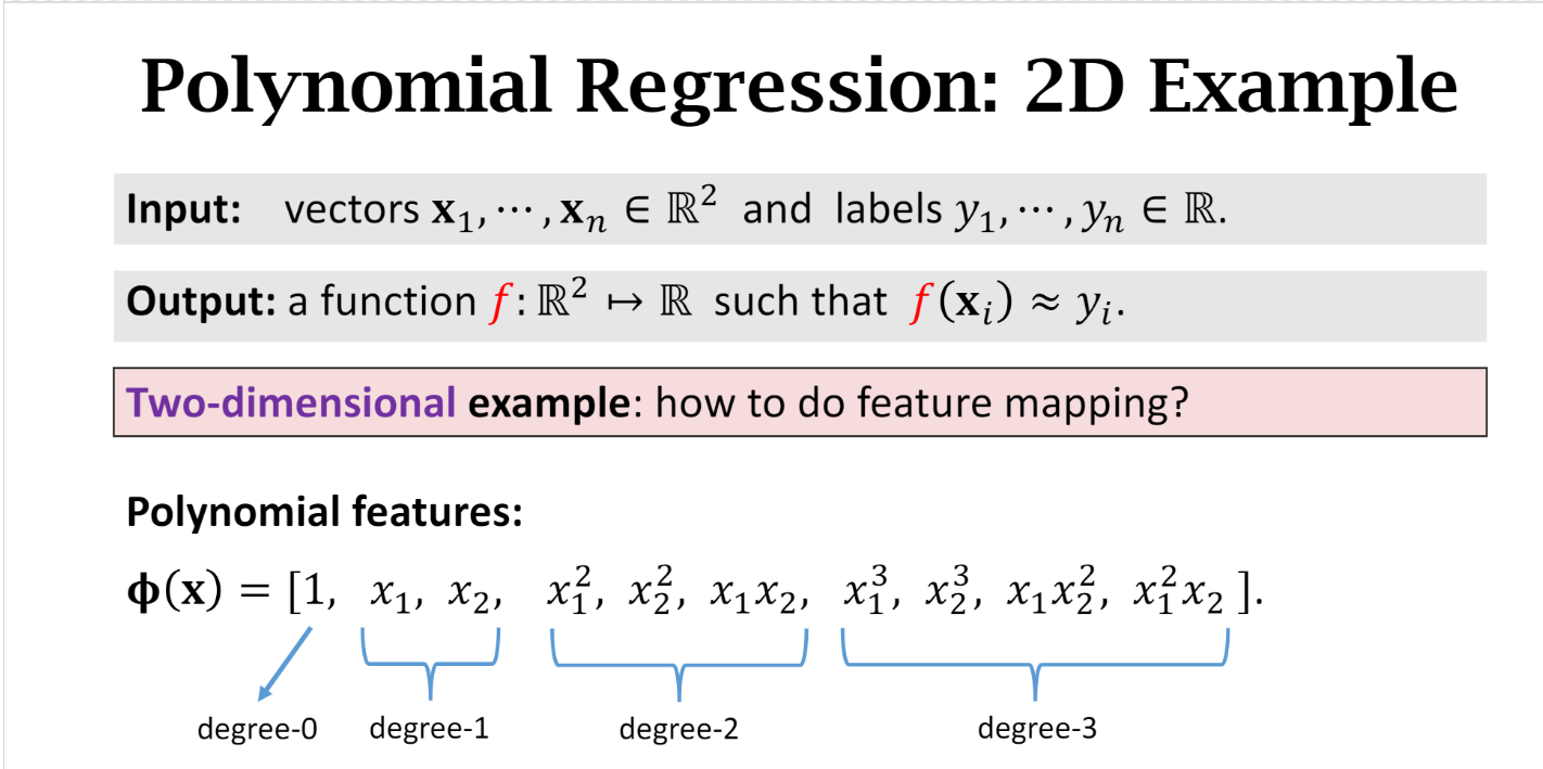
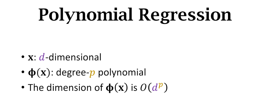
Regression and Hyper-parameter
Naive Cross-Validation
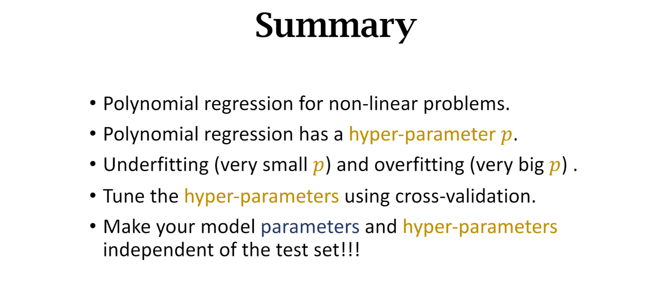
Hyper-Parameter Tuning
Cross-Validation to determine the best Parameter, for example: using different degree k in polynomial regression. Then, find the best θ for each k, and use cross-validation to find the best θ with the lowest loss function. Then, we can know the corresponded k.
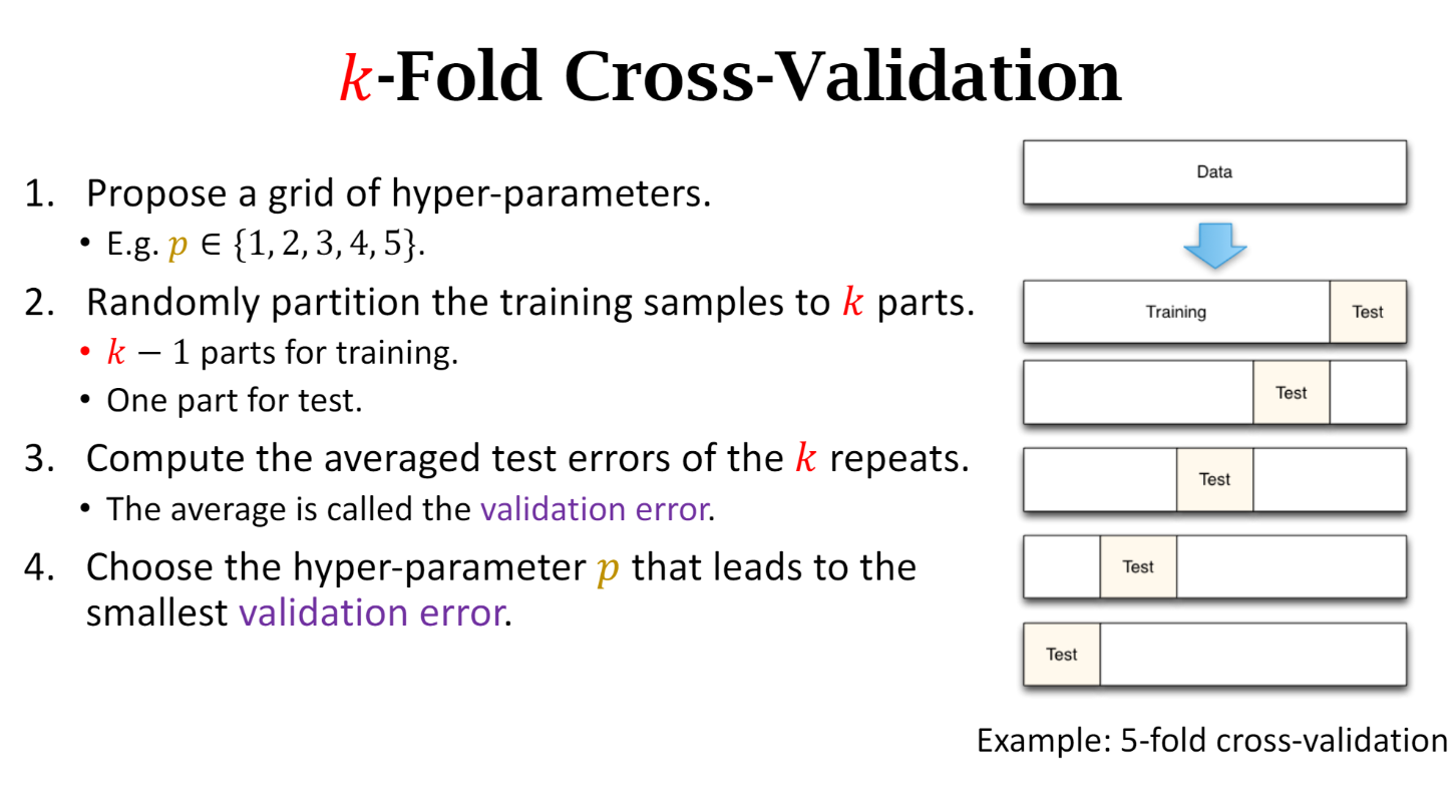
k-fold cross-validation
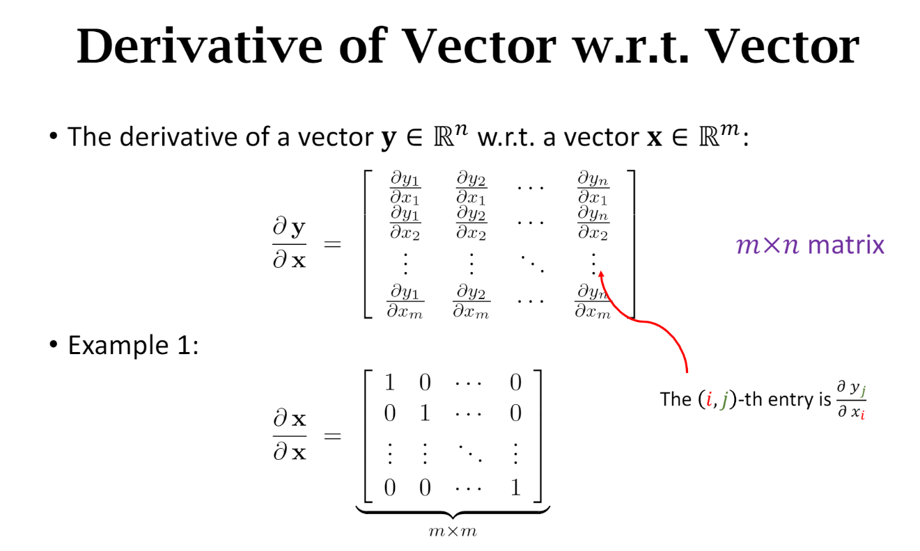
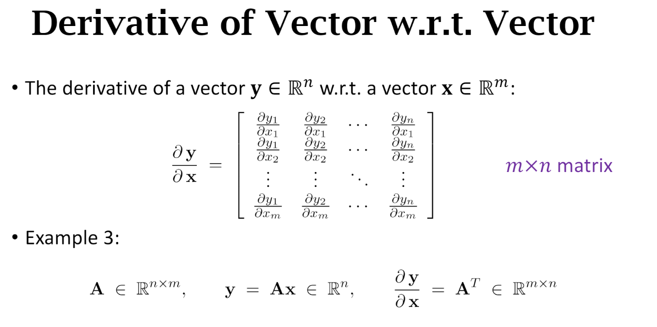
Derivative of Vector
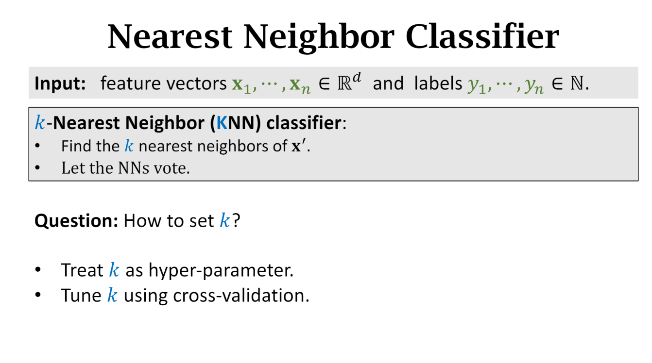
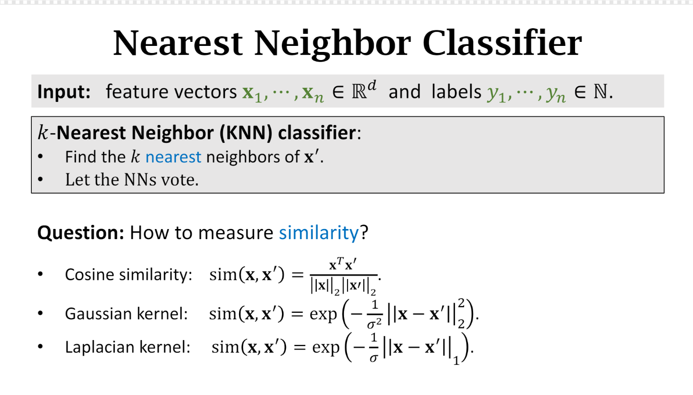
KNN
k is the hyper-parameter for tuning: cross-validation
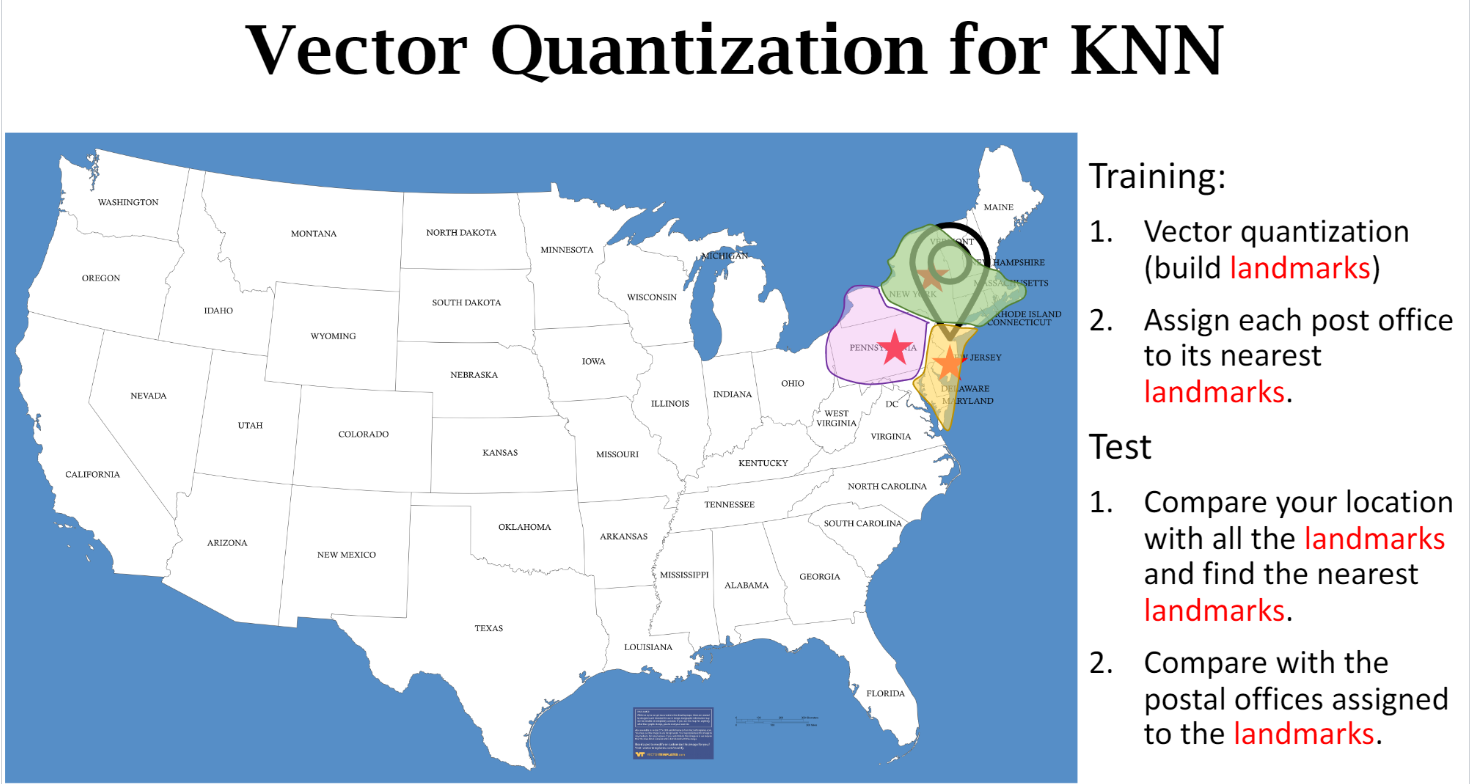
Efficient KNN:
先选取landmarks,相当于cluster;然后找最近的landmark, 然后再在最近的landmark cluster里面找最近的点。
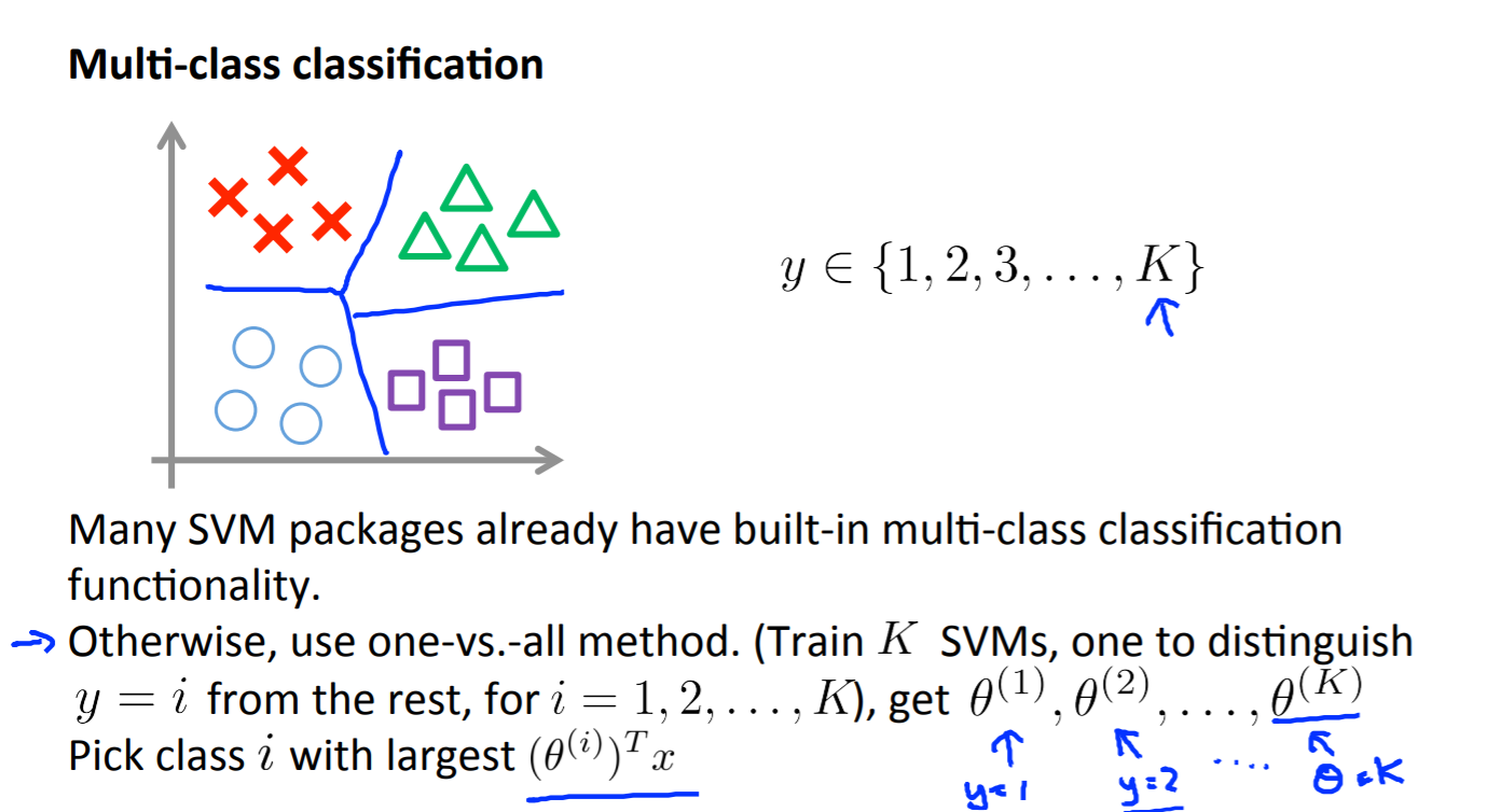
SVM
需要指出 C, choice of kernel function
one vs all, 得到 θ1,…,θn; then choose the largest value of max(i) θi*x + b
Decision Tree and Random Forest:
Decision Tree
决策树学习采用的是自顶向下的递归方法, 其基本思想是以信息熵为度量构造一棵熵值 下降最快的树,到叶子节点处的熵值为零, 此时每个叶节点中的实例都属于同一类。
bootstrap
Bootstraping的名称来自成语“pull up by your own bootstraps”,意思是依靠你自己的资源,称为自助法,它是一种有放回的抽样方法. “拔靴法”: 从手上有限的资料, 产生不同的副本, 来模拟不一样的资料. 从已知大小为 N 的数据集 D 中, 进行 t=1,2,…,T 的过程: 进行有放回的采样, 得到 N′ 大小的数据集 Dt , 从 A{D} 中建立分类器 gt (ID3、C4.5、CART、SVM、Logistic回归等) 重复上述步骤, 得到 m 个分类器, G=Uniform(gt) 作用: 通过投票/平均, 降低变化variance 与决策树恰好相反, 决策树的作用, 是使variance变大, 对数据敏感.

决策树的优缺点
优点: 决策树对训练属于有很好的分类能力, 缺点: 但对未知的测试数据未必有好的分类能力,泛化 能力弱,即可能发生过拟合现象。剪枝,随机森林
随机森林
随机森林能够解决, 决策树的过拟合问题. 随机森林用训练集生成多个(非常深的)决策树.在预测时, 每个树的都会预测一个结果, 每个结果加权表决, 来避免过拟合. 例如, 如果你训练了3个树, 其中有2个树的结果是A, 1个数的结果是B, 那么最终结果会是A。
Random Forest classifiers work around that limitation by creating a whole bunch of decision trees (hence “forest”) — each trained on random subsets of training samples (drawn with replacement) and features (drawn without replacement) — and have the decision trees work together to make a more accurate classification.
信息熵,information entropy:-p*log(p); 如果可取数目较多的属性有所偏好,导致分支过于细化。 增益率:信息增益/IV(可取数值越大,值越大) 基尼系数:Gini(D) = 1- (+)p^2 随机抽取两个样本,其类别标记不一致的概率。
- 不同的子数据集,有放回的抽取
- 不同的特征子集,可能有重复,可以选取部分
Ensemble Learning: 集成学习
数据集大 划分成多个小数据集,学习多个模型进行组合 数据集小 利用Bootstrap方法进行抽样,得到多个数据集,分别训练多个模型再进行组合
Bagging
bootstrap aggregating :自助法,有放回的抽样
在Bagging方法中,利用bootstrap方法从整体数据集中采取有放回抽样得到N个数据集,在每个数据集上学习出一个模型,最后的预测结果利用N个模型的输出得到,具体地:分类问题采用N个模型预测投票的方式,回归问题采用N个模型预测平均的方式
Boosting
算法思想:首先从训练集初始权重训练出一个弱学习器1,根据弱学习器的学习误差率表现来更新训练样本的权重,使得之前弱学习器学习误差率高的训练样本点的权重变高,使得这些误差率高的店在后面的弱学习器2中得到更多的重视。然后基于调整权重后的训练集来训练弱学习器2,如此重复进行,知道弱学习器数达到预定的数目T,最终将这T个弱学习器通过集合策略进行整合,最终得到强学习器
Details
Matrix multiplication
Associative. (A∗B)∗C=A∗(B∗C)
Inverse
The inverse of a matrix A is denoted A−1. Multiplying by the inverse results in the identity matrix.
A non square matrix does not have an inverse matrix. We can compute inverses of matrices in octave with the pinv(A) function [1] and in matlab with the inv(A) function. Matrices that don’t have an inverse are singular or degenerate.
| A | = 0 奇异矩阵,没有逆矩阵 |
Gradient Descent
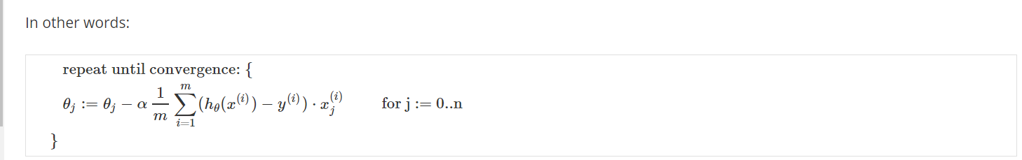
θ:=θ−α∇J(θ)
Diagnostics
A typical rule of thumb when running diagnostics is:
- More training examples fixes high variance but not high bias.
- Fewer features fixes high variance but not high bias.
- Additional features fixes high bias but not high variance.
- The addition of polynomial and interaction features fixes high bias but not high variance.
- When using gradient descent, decreasing lambda can fix high bias and increasing lambda can fix high variance (lambda is the regularization parameter).
- When using neural networks, small neural networks are more prone to under-fitting and big neural networks are prone to over-fitting. Cross-validation of network size is a way to choose alternatives.
SVM vs Logistic
Logistic Regression vs. SVMs If n is large (relative to m), then use logistic regression, or SVM without a kernel (the “linear kernel”)
If n is small and m is intermediate, then use SVM with a Gaussian Kernel
If n is small and m is large, then manually create/add more features, then use logistic regression or SVM without a kernel.
In the first case, we don’t have enough examples to need a complicated polynomial hypothesis. In the second example, we have enough examples that we may need a complex non-linear hypothesis. In the last case, we want to increase our features so that logistic regression becomes applicable.
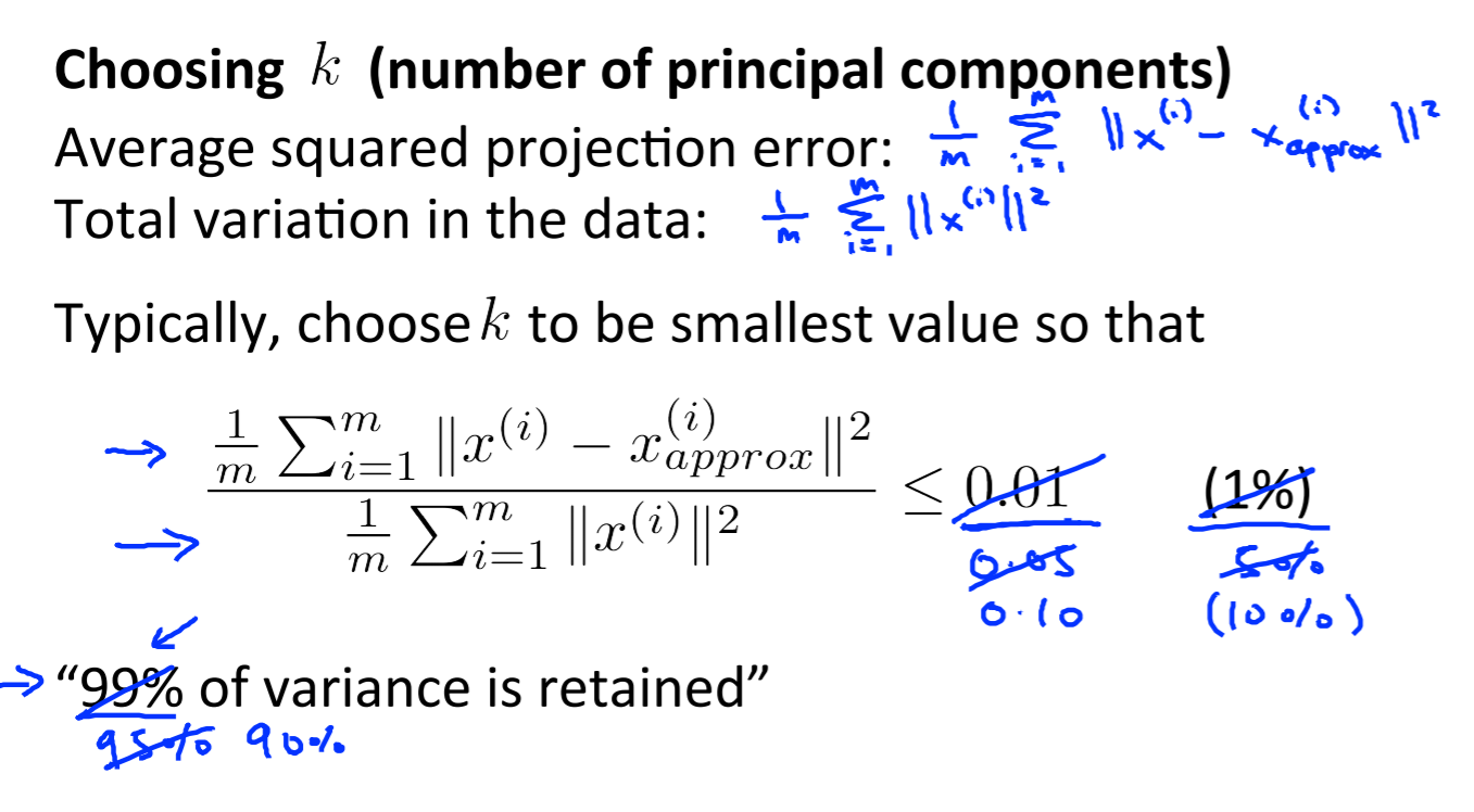
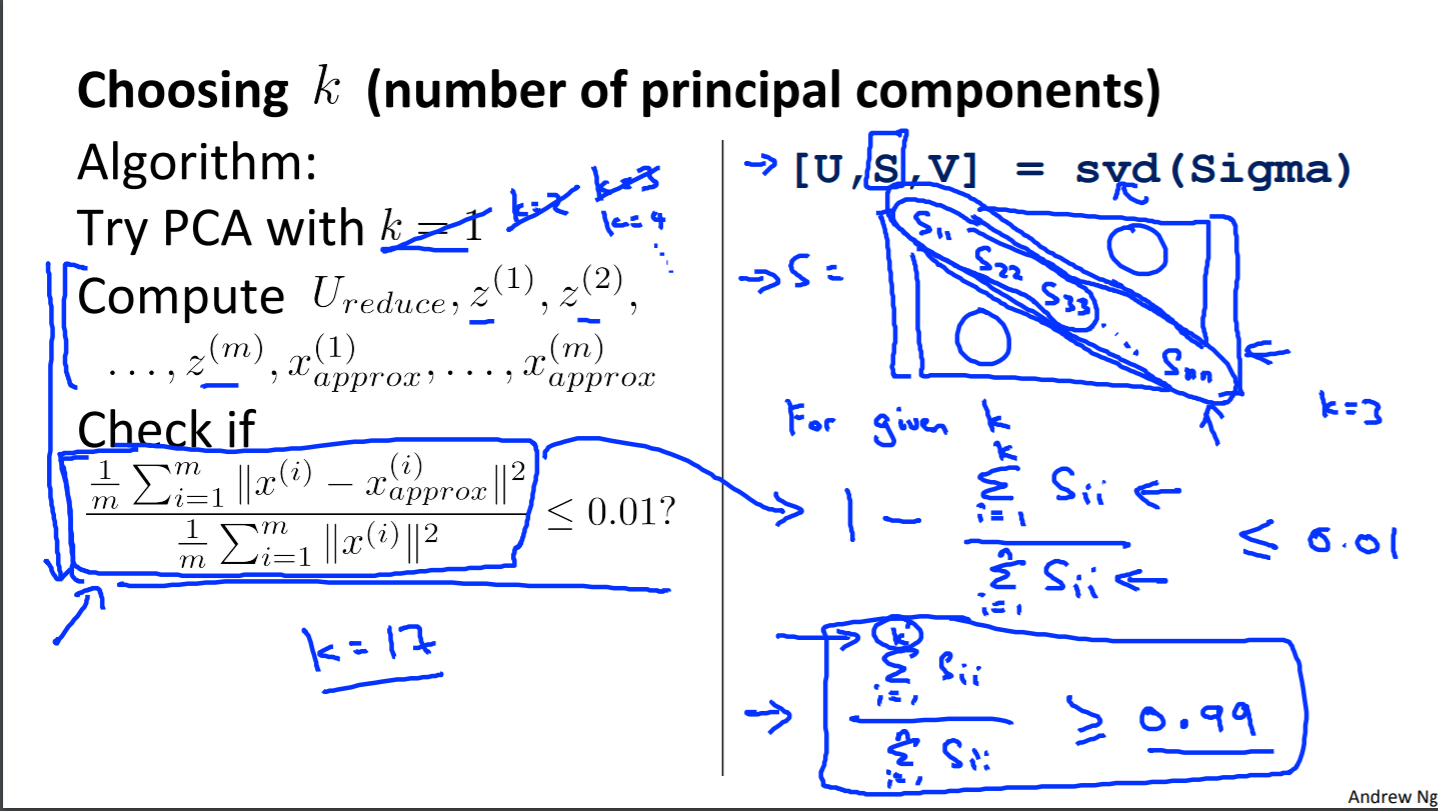
Principle Component Analysis PCA
Find a vector!! Reduce 3D to 2D
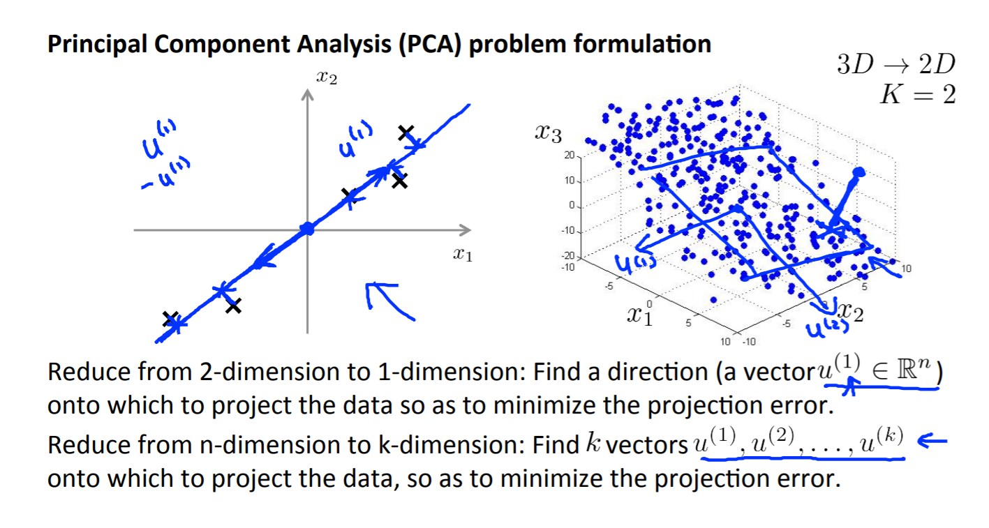
Projection Error: 到这个线的距离,或者这个平面的距离
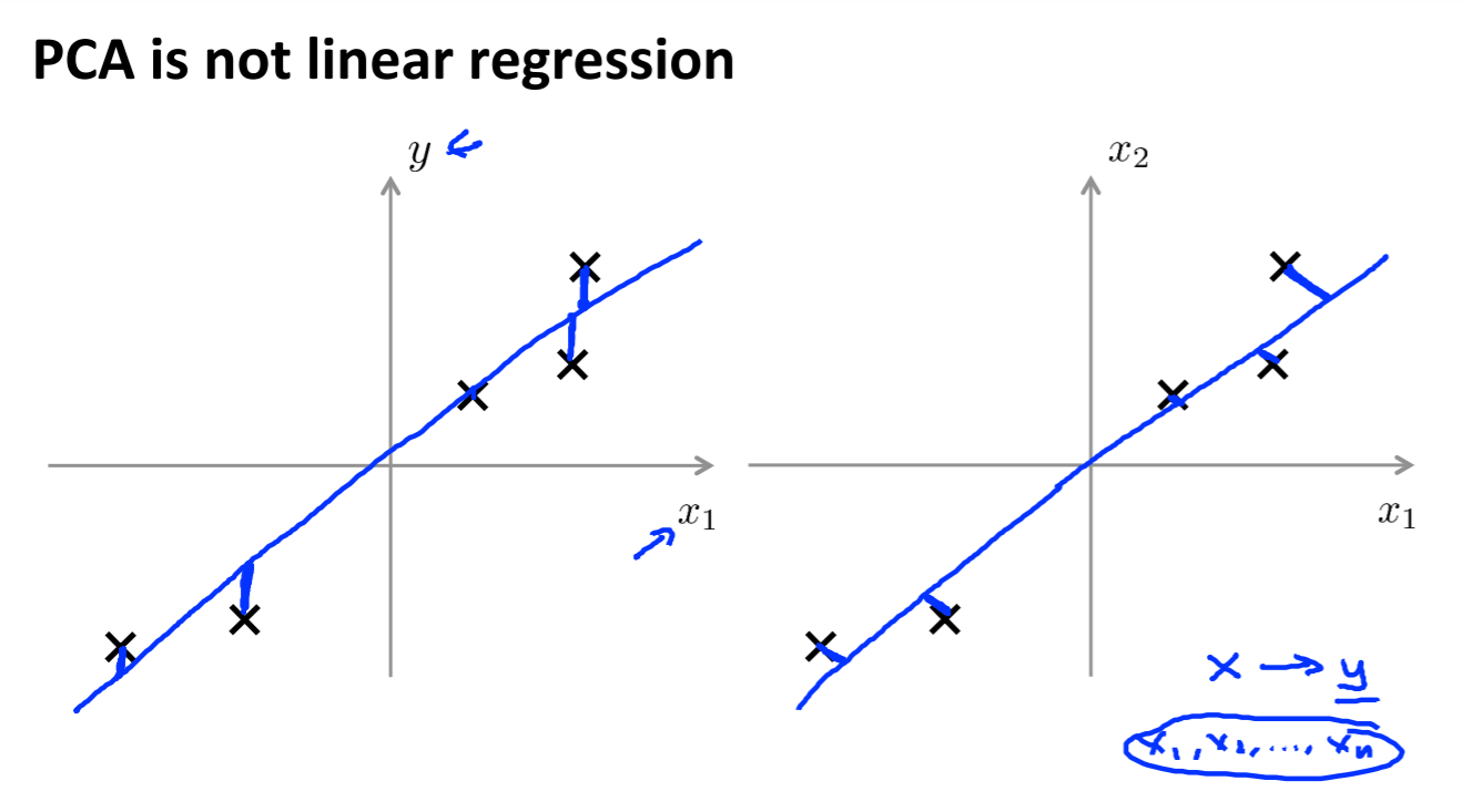
左边是Linear Regression, 右边是 PCA
Mean Normalization and Feature Scaling
SVD: singular value decomposition
Reduce data from n-dimensions to k-dimensions
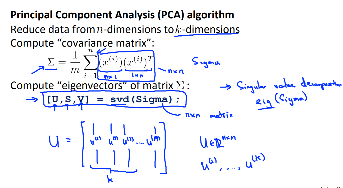
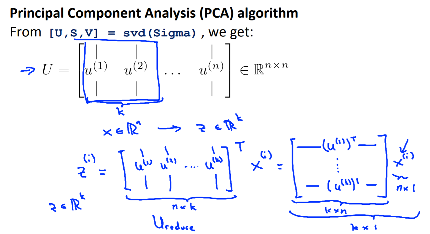
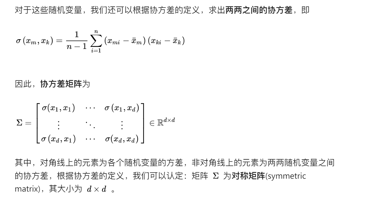
z = U(T)x; U is n*n, 选取k个向量,竖着的,这样就能将n维降低到k维
协方差矩阵 covariance matrix
各个维度的相关性,样品特征均值化后,各特征方差一样。计算得到的协方差矩阵,其中元素的值越大,则说明对应下标的特征之间相关性更高。
用来PCA 的 SVD分解